测试报告
- AMD EPYC Rome VASP 测试
- Gromacs
- vasp6 gpu 测试
- Gromacs-2021.3 (比较常用GPU队列)
- Desmond_2022-4在HPC上的表现和批量化MD操作
- 集群运行Numpy程序的测试实践与注意事项
AMD EPYC Rome VASP 测试
周健 2019.11.18
测试算例
Ruddlesden-Popper 钛酸锶 Sr4Ti3O10,305个原子。
输入文件
SYSTEM = STO

PREC=A

ENCUT=520
EDIFF=1E-6

ADDGRID=.T.

ISMEAR= 1
SIGMA=0.2

LWAVE=.F.
LCHARG=.F.

NELMIN=4
NELM=100
LREAL=Auto

K-Points
0
Gamma
2 2 1
0 0 0
eScience中心测试,软件版本:VASP5.4.4 Intel 2018,CUDA 10.1.243
| 队列信息 | CPU 核数 | Elapsed time (s) | scf次数 | E0 in OSZICAR |
|---|---|---|---|---|
| e5v3ib队列,2*Intel Xeon E5-2680 v3 (12 Cores 2.50 GHz) 256 G RAM | 24 | 6676 | 23 | -.23554005E+04 |
| e52682v4opa队列, 2*Intel Xeon E5-2682 v4 (16 Cores, 2.50 GHz) | 32 | 5967 | 23 | -.23554005E+04 |
| 6140ib队列, 4*Intel Xeon Gold 6140 (18 Cores, 2.30 GHz) 384 G RAM | 72 | 2080 | 23 | -.23554005E+04 |
| 6140ib队列, 4*Intel Xeon Gold 6140 (18 Cores, 2.30 GHz) 384 G RAM | 36 | 2456 | 23 | -.23554005E+04 |
| 6140ib队列, 4*Intel Xeon Gold 6140 (18 Cores, 2.30 GHz) 384 G RAM | 18 | 5005 | 23 | -.23554005E+04 |
| 7702队列, 2*AMD EPYC 7702 (64 Cores, 256MB Cache, 2.0 GHz) 256 G RAM | 32 | 5034 | 23 | -.23554005E+04 |
| 7702队列, 2*AMD EPYC 7702 (64 Cores, 256MB Cache, 2.0 GHz) 256 G RAM | 64 | 3663 | 22 | -.23554005E+04 |
| 7702队列, 2*AMD EPYC 7702 (64 Cores, 256MB Cache, 2.0 GHz) 256 G RAM | 128 | 4401 | 23 | -.23554005E+04 |
| 7502队列, 2*AMD EPYC 7502 (32 Cores, 128MB Cache, 2.5 GHz) 256 G RAM | 32 | 5290 | 23 | -.23554005E+04 |
| 7502队列, 2*AMD EPYC 7502 (32 Cores, 128MB Cache, 2.5 GHz) 256 G RAM | 64 | 4176 | 22 | -.23554005E+04 |
| 62v100ib队列,2*Intel Xeon Gold 6248 (20 Cores, 27.5MB Cache, 2.50 GHz) 768 GB RAM,8*NVIDIA Tesla V100 SXM2 32GB (5120 CUDA Cores 1290MHz, 32GB HBM2 876MHz 4096-bit 900 GB/s, NVLink, PCI-E 3.0 x16) | 1CPU 1GPU | 3053 | 23 | -.23554005E+04 |
校计算中心测试,软件版本:VASP 5.4.4 Intel 2017,CUDA 10.1.168
| 队列信息 | CPU/GPU | Elapsed time (s) | scf次数 | E0 in OSZICAR |
|---|---|---|---|---|
| fat_384队列,4*Intel Xeon Gold 6248 (20 Cores, 2.50 GHz) 384 G RAM | 20 | 5326.949 | 23 | -.23554005E+04 |
| fat_384队列,4*Intel Xeon Gold 6248 (20 Cores, 2.50 GHz) 384 G RAM | 40 | 3105.863 | 23 | -.23554005E+04 |
| fat_384队列,4*Intel Xeon Gold 6248 (20 Cores, 2.50 GHz) 384 G RAM | 80 | 2896.237 | 21 | -.23554005E+04 |
| gpu_v100队列,8 X TESLA V100 NVLink GPU,2 X CPU intel Xeon Gold 6248, 20核,2.5GHz, 768GB 内存 | 1/1 | 3202.687 | 23 | -.23554005E+04 |
| gpu_v100队列,8 X TESLA V100 NVLink GPU,2 X CPU intel Xeon Gold 6248, 20核,2.5GHz, 768GB 内存 | 2/2 | 2244.153 | 23 | -.23554005E+04 |
| gpu_v100队列,8 X TESLA V100 NVLink GPU,2 X CPU intel Xeon Gold 6248, 20核,2.5GHz, 768GB 内存 | 4/4 | 1379.651 | 23 | -.23554005E+04 |
| gpu_v100队列,8 X TESLA V100 NVLink GPU,2 X CPU intel Xeon Gold 6248, 20核,2.5GHz, 768GB 内存 | 8/8 | 1214.461 | 23 | -.23554005E+04 |
结论
- AMD EPYC Rome 比 Intel V3/V4 快一些,但比 Intel Gold 系列慢许多
- 核心太多对于VASP并不有利
Gromacs
注意:为了保证GPU性能, 在没有特殊要求的情况下,请使用2021版本的Gromacs,并用GPU计算所有的相互作用。没特殊要求的话请看第三部分。
1. Gromacs-2018.8
说明:
Gromacs使用CPU计算成键相互作用,使用GPU计算非键相互作用。
编译环境:
gcc/7.4.0
cmake/3.16.3
ips/2017u2
fftw/3.3.7-iccifort-17.0.6-avx2
cuda/10.0.130
软件信息:
GROMACS version:    2018.8
Precision:          single
Memory model:       64 bit
MPI library:        MPI
OpenMP support:     enabled (GMX_OPENMP_MAX_THREADS = 64)
GPU support:        CUDA
SIMD instructions:  AVX2_256
FFT library:        fftw-3.3.7-avx2-avx2_128
CUDA driver:        11.40
CUDA runtime:       10.0
测试算例:
ATOM  102808(464 residues, 9nt DNA, 31709 SOL, 94 NA, 94 CL)
nsteps      = 25000000     ;50 ns
eScience中心GPU测试: 所有GPU节点使用单个GPU进行模拟。
2. Gromacs-2021.3
说明:
使用的是集群自带的容器化(singularity)的gromacs-2021.3. Gromacs使用CPU计算成键相互作用,使用GPU计算非键相互作用。
文件位置
/fs00/software/singularity-images/ngc_gromacs_2021.3.sif
提交代码
#BSUB -q GPU_QUEUE
#BSUB -gpu "num=1"
export OMP_NUM_THREADS="$LSB_DJOB_NUMPROC"
SINGULARITY="singularity run --nv /fs00/software/singularity-images/ngc_gromacs_2021.3.sif"
${SINGULARITY} gmx mdrun -nb gpu -deffnm <NAME>
软件信息:
GROMACS version:    2021.3-dev-20210818-11266ae-dirty-unknown
Precision:          mixed
Memory model:       64 bit
MPI library:        thread_mpi
OpenMP support:     enabled (GMX_OPENMP_MAX_THREADS = 64)
GPU support:        CUDA
SIMD instructions:  AVX2_256
FFT library:        fftw-3.3.9-sse2-avx-avx2-avx2_128-avx512
CUDA driver:        11.20
CUDA runtime:       11.40
测试算例:
ATOM  102808(464 residues, 9nt DNA, 31709 SOL, 94 NA, 94 CL)
nsteps      = 25000000     ;50 ns
eScience中心GPU测试: 所有GPU节点使用单个GPU进行模拟。
3. Gromacs-2021.3(全部相互作用用GPU计算)
说明:
由于从2019版本开始,不同的相互作用慢慢都可以在GPU上进行运算,2021版本已经可以将所有模拟的计算用GPU来模拟,所以尝试用GPU进行所有相互作用的运算。
文件位置
/fs00/software/singularity-images/ngc_gromacs_2021.3.sif
提交代码
#BSUB -q GPU_QUEUE
#BSUB -gpu "num=1"
export OMP_NUM_THREADS="$LSB_DJOB_NUMPROC"	# 需要,否则会占用所有CPU,反而导致速度变慢
SINGULARITY="singularity run --nv /fs00/software/singularity-images/ngc_gromacs_2021.3.sif"
${SINGULARITY} gmx mdrun -nb gpu -bonded gpu -update gpu -pme gpu -pmefft gpu -deffnm <NAME>	# 设置所有的运算用GPU进行
测试算例:
ATOM  102808(464 residues, 9nt DNA, 31709 SOL, 94 NA, 94 CL)
nsteps      = 25000000     ;50 ns
eScience中心GPU测试: 所有GPU节点使用单个GPU进行模拟。
结论:
- 对于GPU节点来说,如果使用GPU+CPU混合运算,主要限制的速度的会是CPU,所以应该尽可能使用GPU进行相互作用的计算。
补充信息
每个GPU队列带有的CPU核数
| Queue | CPU Core |
|---|---|
| 72rtxib | 4 |
| 722080tiib | 4 |
| 723090ib | 6 |
| 62v100ib | 5 |
| 83a100ib | 8 |
vasp6 gpu 测试
Gromacs-2021.3 (比较常用GPU队列)
4. Gromacs-2021.3 (比较常用GPU队列)
说明:
使用Singularity容器解决方案,调用/fs00/software/singularity-images/ngc_gromacs_2021.3.sif完成Gromacs的能量最小化(em)、平衡模拟(nvt、npt)以及成品模拟(md)在公共共享100%GPU队列722080tiib、72rtxib、723090ib的表现。
队列情况:
| 队列 | 节点数 | 每节点CPU | 每节点内存(GB) | 平均每核内存(GB) | CPU主频(GHz) | 每节点GPU数量 | 每GPU显存(GB) | 浮点计算理论峰值(TFLOPS) |
|---|---|---|---|---|---|---|---|---|
| 83a100ib | 1 | 64 | 512 | 8 | 2.6 | 8 | 40 | 双精度:82.92 单精度:------ |
| 723090ib | 2 | 48 | 512 | 10.7 | 2.8 | 8 | 24 | 双精度:4.30 单精度:569.28 |
| 722080tiib | 4 | 16 | 128 | 8.0 | 3.0 | 4 | 11 | 双精度:3.07 单精度:215.17 |
| 72rtxib | 3 | 16 | 128 | 8.0 | 3.0 | 4 | 24 | 双精度:2.30 单精度:195.74 |
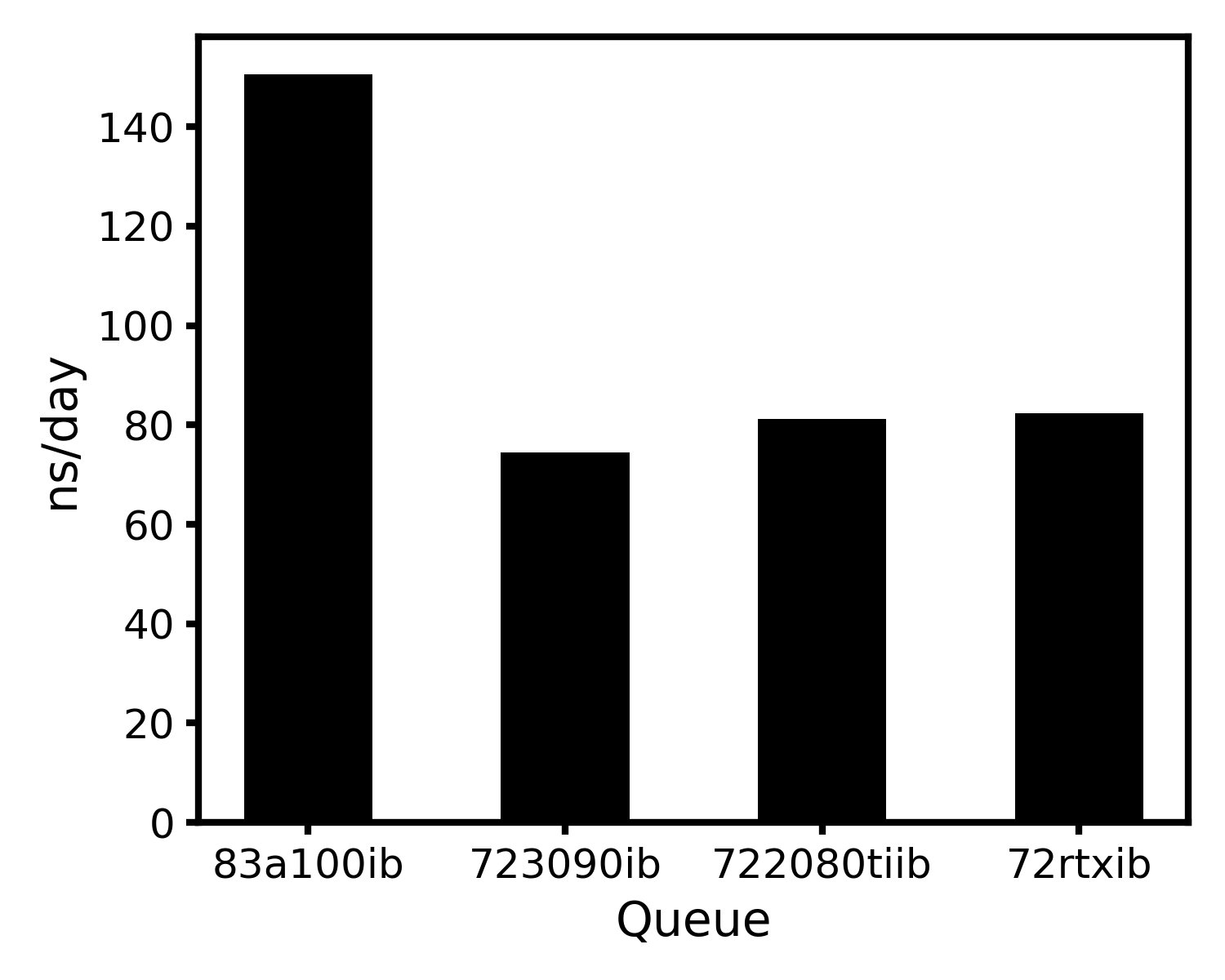
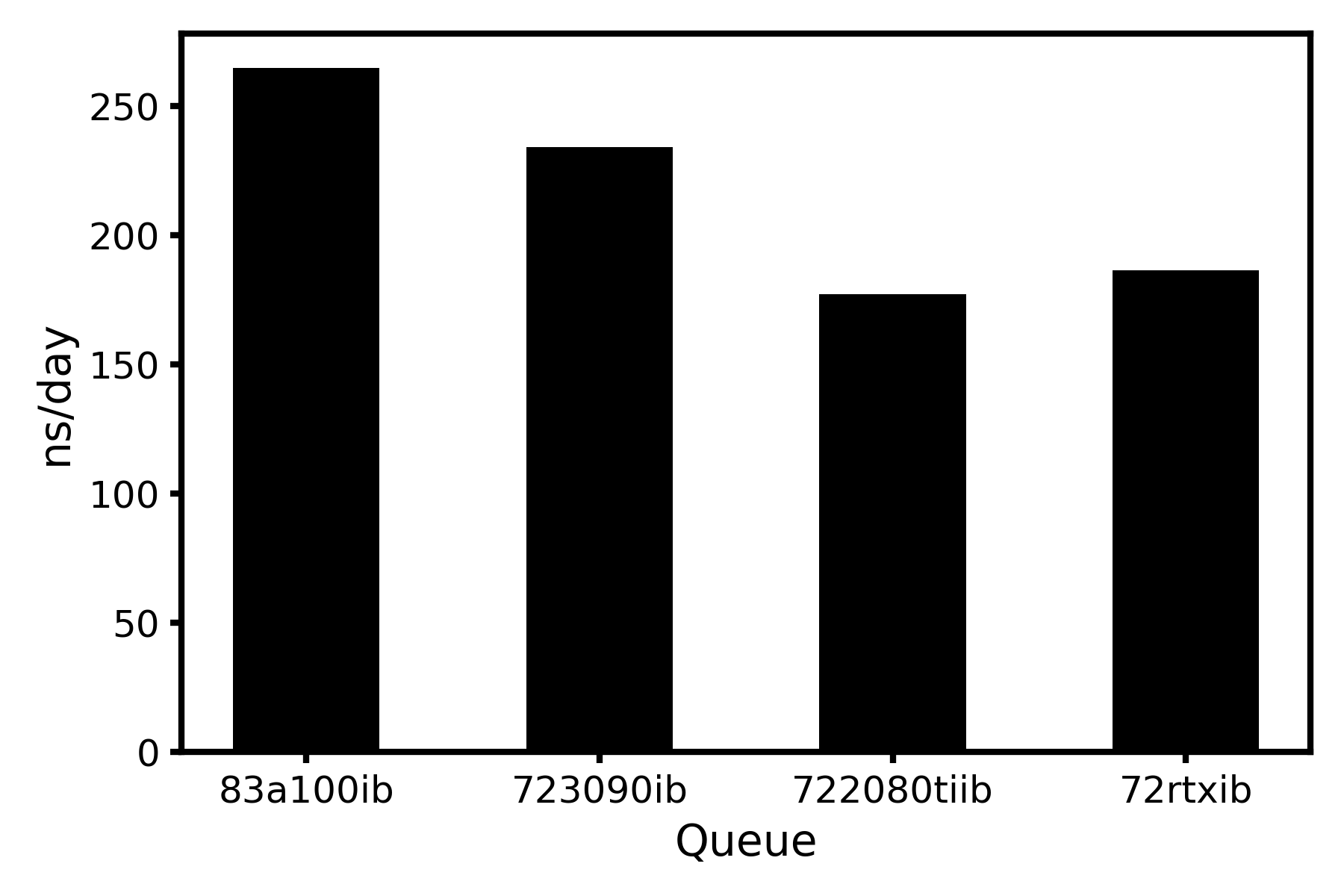
前人关于Gromacs-2021.3(全部相互作用用GPU计算)的测试报告中,尝试用GPU来模拟102808个原子体系(464 residues, 9nt DNA, 31709 SOL, 94 NA, 94 CL)50 ns内所有相互作用的运算,结果表明83a100ib(250 ns/day以上)>723090ib(220 ns/day以上)>722080tiib(170 ns/day以上)>72rtxib(180 ns/day以上),但83a100ib和723090ib队列常年存在80以上的NJOBS,因此作为成品模拟的前期准备,笔者通常不使用这两个队列。
文件位置:
/fs00/software/singularity-images/ngc\_gromacs\_2021.3.sif
提交代码:
能量最小化(em.lsf)
#BSUB -q 72rtxib
#BSUB -gpu "num=1"
export OMP_NUM_THREADS="$LSB_DJOB_NUMPROC"
SINGULARITY="singularity run --nv /fs00/software/singularity-images/ngc_gromacs_2021.3.sif"
${SINGULARITY} gmx grompp -f minim.mdp -c 1aki_solv_ions.gro -p topol.top -o em.tpr
${SINGULARITY} gmx mdrun -nb gpu -ntmpi 2 -deffnm em
平衡模拟(nvt)
#BSUB -q 72rtxib
#BSUB -gpu "num=1"
export OMP_NUM_THREADS="$LSB_DJOB_NUMPROC"
SINGULARITY="singularity run --nv /fs00/software/singularity-images/ngc_gromacs_2021.3.sif"
${SINGULARITY} gmx grompp -f nvt.mdp -c em.gro -r em.gro -p topol.top -o nvt.tpr
${SINGULARITY} gmx mdrun -nb gpu -ntmpi 2 -deffnm nvt
平衡模拟(npt)
#BSUB -q 72rtxib
#BSUB -gpu "num=1"
export OMP_NUM_THREADS="$LSB_DJOB_NUMPROC"
SINGULARITY="singularity run --nv /fs00/software/singularity-images/ngc_gromacs_2021.3.sif"
${SINGULARITY} gmx grompp -f npt.mdp -c nvt.gro -r nvt.gro -t nvt.cpt -p topol.top -o npt.tpr
${SINGULARITY} gmx mdrun -nb gpu -ntmpi 2 -deffnm npt
成品模拟(md)
#BSUB -q 723090ib
#BSUB -gpu "num=1"
export OMP_NUM_THREADS="$LSB_DJOB_NUMPROC"
SINGULARITY="singularity run --nv /fs00/software/singularity-images/ngc_gromacs_2021.3.sif"
${SINGULARITY} gmx grompp -f md.mdp -c npt.gro -t npt.cpt -p topol.top -o md_0_1.tpr
${SINGULARITY} gmx mdrun -nb gpu -bonded gpu -update gpu -pme gpu -pmefft gpu -deffnm md_0_1
成品模拟(md)
也可以参照以下命令进行修改,以作业脚本形式进行提交:
#BSUB -q 723090ib
#BSUB -gpu "num=1"
export OMP_NUM_THREADS="$LSB_DJOB_NUMPROC"
SINGULARITY="singularity run --nv /fs00/software/singularity-images/ngc_gromacs_2021.3.sif"
${SINGULARITY} gmx pdb2gmx -f protein.pdb -o protein_processed.gro -water tip3p -ignh -merge all <<< 4
${SINGULARITY} gmx editconf -f protein_processed.gro -o pro_newbox.gro -c -d 1.0 -bt cubic
${SINGULARITY} gmx solvate -cp pro_newbox.gro -cs spc216.gro -o pro_solv.gro -p topol.top
${SINGULARITY} gmx grompp -f ../MDP/ions.mdp -c pro_solv.gro -p topol.top -o ions.tpr
${SINGULARITY} gmx genion -s ions.tpr -o pro_solv_ions.gro -p topol.top -pname NA -nname CL -neutral <<< 13
${SINGULARITY} gmx grompp -f ../MDP/minim.mdp -c pro_solv_ions.gro -p topol.top -o em.tpr
${SINGULARITY} gmx mdrun -v -deffnm em
${SINGULARITY} gmx energy -f em.edr -o potential.xvg <<< "10 0"
${SINGULARITY} gmx grompp -f ../MDP/nvt.mdp -c em.gro -r em.gro -p topol.top -o nvt.tpr
${SINGULARITY} gmx mdrun -deffnm nvt
${SINGULARITY} gmx energy -f nvt.edr -o temperature.xvg <<< "16 0"
${SINGULARITY} gmx grompp -f ../MDP/npt.mdp -c nvt.gro -r nvt.gro -t nvt.cpt -p topol.top -o npt.tpr
${SINGULARITY} gmx mdrun -deffnm npt
${SINGULARITY} gmx energy -f npt.edr -o pressure.xvg <<< "18 0"
${SINGULARITY} gmx grompp -f ../MDP/md.mdp -c npt.gro -t npt.cpt -p topol.top -o md.tpr
${SINGULARITY} gmx mdrun -v -deffnm md
${SINGULARITY} gmx rms -f md.xtc -s md.tpr -o rmsd.xvg <<< "4 4"
软件信息:
GROMACS version:    2021.3-dev-20210818-11266ae-dirty-unknown
Precision:          mixed
Memory model:       64 bit
MPI library:        thread_mpi
OpenMP support:     enabled (GMX_OPENMP_MAX_THREADS = 64)
GPU support:        CUDA
SIMD instructions:  AVX2_256
FFT library:        fftw-3.3.9-sse2-avx-avx2-avx2_128-avx512
CUDA driver:        11.20
CUDA runtime:       11.40
测试算例:
ATOM 218234 (401 Protein residues, 68414 SOL, 9 Ion residues)

nsteps = 100000000 ; 200 ns
eScience中心GPU测试: 能量最小化(em)、平衡模拟(nvt、npt)使用1个GPU进行模拟,成品模拟(md)使用1个GPU进行模拟。
| 任务1 | em | nvt | npt | md |
|---|---|---|---|---|
| --- | 72rtxib | 722080tiib | 722080tiib | 723090ib |
| CPU time | 1168.45 | 13960.33 | 42378.71 | |
| Run time | 79 | 1648 | 5586 | 117.428 ns/day 0.204 hour/ns |
| Turnaround time | 197 | 1732 | 5661 | |
| 任务2 | em | nvt | npt | md |
| --- | 72rtxib | 722080tiib | 72rtxib | 722080tiib |
| CPU time | 1399.30 | 15732.66 | 40568.04 | |
| Run time | 93 | 1905 | 5236 | 106.862 ns/day 0.225 hour/ns |
| Turnaround time | 181 | 1991 | 5479 | |
| 任务3 | em | nvt | npt | md |
| --- | 72rtxib | 72rtxib | 72rtxib | 72rtxib |
| CPU time | 1368.11 | 5422.49 | 5613.74 | |
| Run time | 92 | 355 | 366 | 103.213 ns/day 0.233 hour/ns |
| Turnaround time | 180 | 451 | 451 | |
| 任务4 | em | nvt | npt | md |
| --- | 72rtxib | 72rtxib | 72rtxib | 722080tiib |
| CPU time | 1321.15 | 5441.60 | 5618.87 | |
| Run time | 89 | 356 | 369 | 111.807 ns/day 0.215 hour/ns |
| Turnaround time | 266 | 440 | 435 | |
| 任务5 | em | nvt | npt | md |
| --- | 72rtxib | 72rtxib | 72rtxib | 72rtxib |
| CPU time | 1044.17 | 5422.94 | 5768.44 | |
| Run time | 72 | 354 | 380 | 110.534 ns/day 0.217 hour/ns |
| Turnaround time | 162 | 440 | 431 | |
| 任务6 | em | nvt | npt | md |
| --- | 723090ib | 723090ib | 723090ib | 723090ib |
| CPU time | 1569.17 | 7133.74 | 6677.25 | |
| Run time | 81 | 326 | 325 | 114.362 ns/day 0.210 hour/ns |
| Turnaround time | 75 | 320 | 300 | |
| 任务7 | em | nvt | npt | md |
| --- | 723090ib | 723090ib | 723090ib | 722080tiib |
| CPU time | 1970.56 | 5665.71 | 6841.73 | |
| Run time | 91 | 253 | 327 | 111.409 ns/day 0.215 hour/ns |
| Turnaround time | 123 | 251 | 328 | |
| 任务8 | em | nvt | npt | md |
| --- | 72rtxib | 72rtxib | 72rtxib | 72rtxib |
| CPU time | 1234.24 | 5540.59 | 5528.91 | |
| Run time | 108 | 363 | 370 | 114.570 ns/day 0.209 hour/ns |
| Turnaround time | 85 | 364 | 363 | |
| 任务9 | em | nvt | npt | md |
| --- | 723090ib | 723090ib | 723090ib | 723090ib |
| CPU time | 2016.10 | 7633.83 | 7983.58 | |
| Run time | 93 | 342 | 361 | 115.695 ns/day 0.207 hour/ns |
| Turnaround time | 130 | 377 | 356 | |
| 任务10 | em | nvt | npt | md |
| --- | 723090ib | 723090ib | 723090ib | 72rtxib |
| CPU time | 1483.84 | 7025.65 | 7034.90 | |
| Run time | 68 | 317 | 333 | 102.324 ns/day 0.235 hour/ns |
| Turnaround time | 70 | 319 | 316 |
结论:
-
能量最小化(em)在任务较少的722080tiib和72rtxib队列中,Run time分别为88.83 ± 12.45和83.25 ± 11.44s;
-
平衡模拟(nvt)任务在722080tiib、72rtxib和723090ib队列中,Run time分别为1776.50 ± 181.73、357.00 ± 4.08和309.50 ± 39.06 s;
-
平衡模拟(npt)任务在722080tiib、72rtxib和723090ib队列中,Run time分别为5411.00 ± 247.49、371.25 ± 6.08和336.50 ± 16.68 s;
-
原子数218234的 200 ns成品模拟(md)任务在722080tiib、72rtxib、和723090ib队列中,性能表现差别不大,分别为110.03 ± 2.75、115.83 ± 1.54和107.66 ± 5.90 ns/day。
-
综上,建议在能量最小化(em)、平衡模拟(nvt、npt)等阶段使用排队任务较少的72rtxib队列 ,建议在成品模拟(md)阶段按照任务数量(从笔者使用情况来看,排队任务数量72rtxib<722080tiib<723090ib<83a100ib)、GPU收费情况(校内及协同创新中心用户:72rtxib队列1.8 元/卡/小时=0.45元/核/小时、722080tiib队列1.2 元/卡/小时=0.3元/核/小时、723090ib队列1.8 元/卡/小时=0.3元/核/小时、83a100ib队列4.8 元/卡/小时=0.3元/核/小时)适当考虑队列。
-
在以上提交代码中,未涉及到Gromacs的并行效率问题(直接“num=4”并不能在集群同时使用4块GPU),感兴趣的同学可以查看http://bbs.keinsci.com/thread-13861-1-1.html以及https://developer.nvidia.com/blog/creating-faster-molecular-dynamics-simulations-with-gromacs-2020/的相关解释。但根据前辈的经验,ATOM 500000以上才值得使用两张GPU加速卡,原因在于Gromacs的并行效率不明显。感兴趣的同学也可以使用Amber的GPU并行加速,但对显卡的要求为3090或者tesla A100。这里提供了GPU=4的gromacs命令:
gmx mdrun -deffnm $file.pdb.md -ntmpi 4 -ntomp 7 -npme 1 -nb gpu -pme gpu -bonded gpu -pmefft gpu -v
Desmond_2022-4在HPC上的表现和批量化MD操作
拳打Amber脚踢Gromacs最终攀上Desmond高峰
一、说明:
笔者在长期受到Amber、Gromacs模拟系统构建的折磨后,痛定思痛决定下载带有GUI美观、完全自动化、一键分析的Desmond。上海科技大学Wang-Lin搭建了Schrödinger中文社区微信群(公众号:蛋白矿工),实现了使用者的互相交流和问答摘录整理,并就Schrödinger软件的使用编写了大量实用脚本。
基于命令行操作的Amber代码包非常适合生物分子体系的模拟,包括AmberTools、Amber两部分。前者免费,但提升生产力的多CPU并行和GPU加速功能需要通过Amber实现,但发展中国家(如中国)可以通过学术申请获得。
同样基于命令行操作的的Gromacs代码包由于上手快、中文教程详尽等优点收到初学者的一致好评,教程可以参考李继存老师博客(http://jerkwin.github.io/)、B站和计算化学公社(http://bbs.keinsci.com/forum.php)等。 初学者跟着教程做就可以(http://www.mdtutorials.com/),深入学习还是推荐大家去看官方的文档。
初识Desmond是使用世界上最贵的分子模拟软件之一的“学术版”Maestro时,它是由D.E.Shaw Research开发的MD代码,但在Schrödinger公司的帮助下实现了GUI图形界面操作。投资界科学家D.E.Shaw顺手还制造l一台用于分子动力学模拟的专业超级计算机Anton2,当然相对于宇宙最快的Gromacs还是差了点(懂得都懂)。学术和非营利机构用户更是可以在D.E.Shaw Research官方网站注册信息,免费获得拥有Maestro界面的Desmond软件。
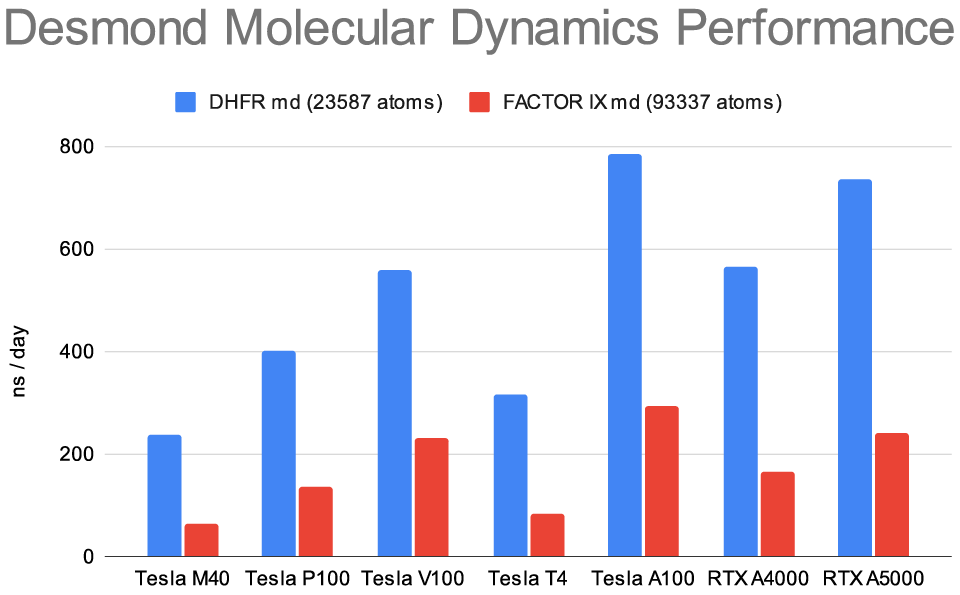
Figure 1: Molecular Dynamics run using default parameters in Schrödinger Suite 2023-1.
二、Desmonds的安装:
在D.E.Shaw Research注册后下载相应软件包,上传到HPC集群个人home下任意位置,随后创建软件文件夹(作为后续安装路径)复制pwd输出的路径内容(笔者为/fsa/home/ljx_zhangzw/software):
mkdir software
pwd
解压安装,进入安装引导界面并按Enter继续进行安装:
tar -xvf Desmond_Maestro_2022.4.tar
cd DESRES_Academic_2022-4_Linux-x86_64
./INSTALL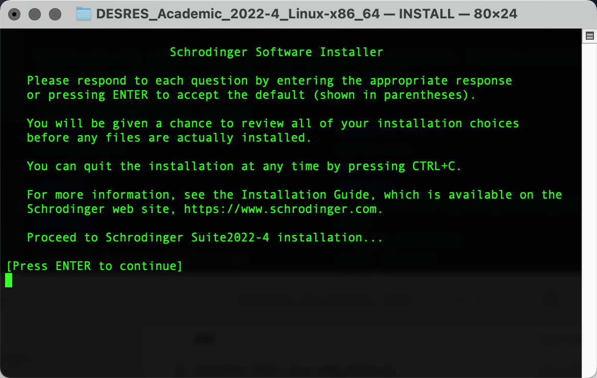
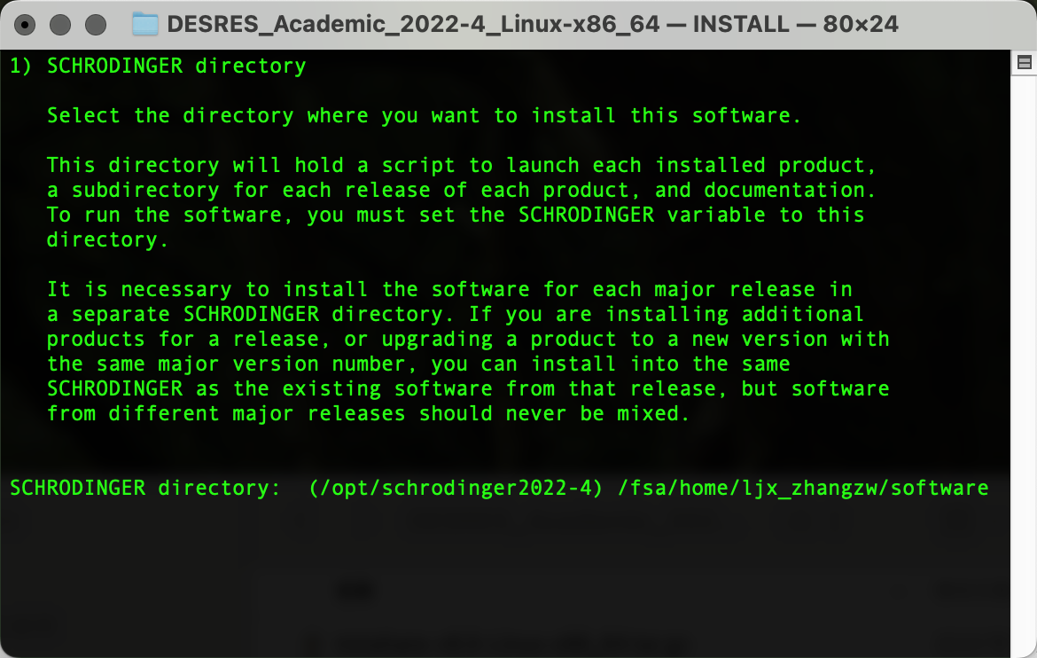
输出以下界面后粘贴复制pwd输出的路径内容,Enter确认为安装路径:
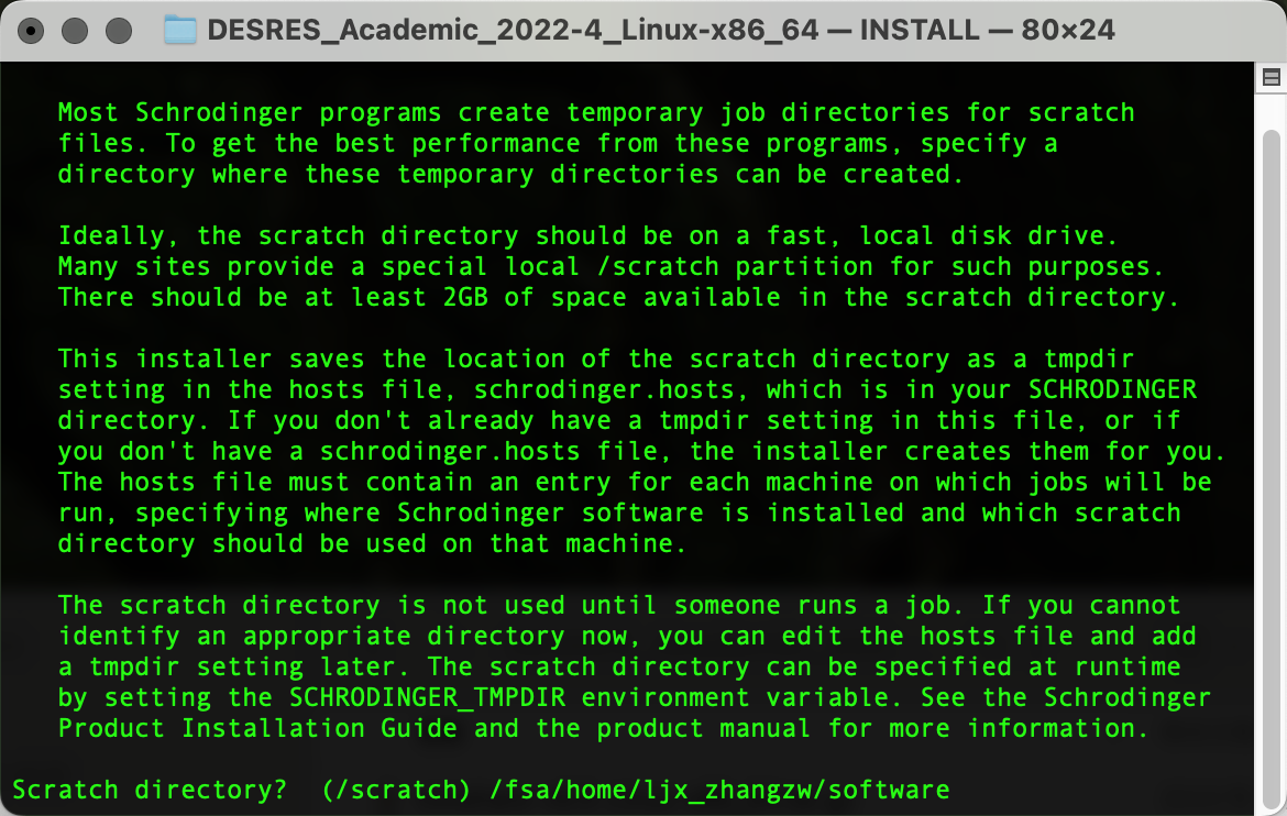
输出以下界面后粘贴复制pwd输出的路径内容,Enter确认为临时文件路径:
输出以下界面后输入y,Enter确认上述两个路径并进行安装:
安装完成后进入安装路径,并写入环境变量:
cd /fsa/home/ljx_zhangzw/software
echo "export Desmond=${PWD}/" >> ~/.bashrc
同时由于Desmond对集群计算中提交任务队列的要求,需要在安装路径修改schrodinger.host以定义GPU信息,示例给出的是83a100ib队列中m001节点信息:
#localhost
name:localhost
temdir:/fsa/home/ljx_zhangzw/software

#HPC
name: HPC
host: m001
queue: LSF
qargs: -q 83a100ib -gpu num=1
tmpdir: /fsa/home/ljx_zhangzw/software
schrodinger: /fsa/home/ljx_zhangzw/software
gpgpu: 0, NVIDIA A100
gpgpu: 1, NVIDIA A100
gpgpu: 2, NVIDIA A100
gpgpu: 3, NVIDIA A100
gpgpu: 4, NVIDIA A100
gpgpu: 5, NVIDIA A100
gpgpu: 6, NVIDIA A100
gpgpu: 7, NVIDIA A100
需要注意的是:
1、修改tmpdir和schrodinger对应路径为自己的安装路径;
2、节点host、队列83a100ib以及显卡信息gpgpu: 0-7, NVIDIA A100自行调整,可以查看HPC的计算资源;
3、对于不同的任务调度系统,Schrödinger公司KNOWLEDGE BASE和蛋白矿工知乎号Q2进行了介绍;
4、截止2023年6月16日,HPC集群可供Desmond使用的计算卡(而非3090、4090等)包括:
| 队列 | GPU | Hostname | 加速卡机时收费 | ||
| e5v3k40ib | 2*Intel Xeon E5-2680v3 2*NVIDIA Tesla K40 12GB 128GB RAM 56Gb FDR InfiniBand |
x001 gpgpu: 0, NVIDIA Tesla K40 gpgpu: 1, NVIDIA Tesla K40 |
校内及协同创新中心用户 1.2 元/卡/小时=0.1元/核/小时 |
1.2 | =0.1 |
| e5v4p100ib | 2*Intel Xeon E5-2660v4 2*NVIDIA Tesla P100 PCIe 16GB 128GB RAM 56Gb FDR InfiniBand |
x002 gpgpu: 0, NVIDIA Tesla P100 gpgpu: 1, NVIDIA Tesla P100 |
校内及协同创新中心用户 1.68 元/卡/小时=0.12元/核/小时 |
||
| 62v100ib | 2*Intel Xeon Gold 6248 8*NVIDIA Tesla V100 SXM2 32GB 768GB RAM 100Gb EDR InfiniBand |
n002 gpgpu: 0, NVIDIA Tesla V100 |
校内及协同创新中心用户 3 元/卡/小时=0.6元/核/小时 |
||
| 72rtxib | AMD EPYC 7302 4*NVIDIA TITAN RTX 24GB 128GB RAM 100Gb HDR100 InfiniBand |
g005 or g006 or g007 gpgpu: 0, NVIDIA TITAN RTX |
校内及协同创新中心用户 1.8 元/卡/小时=0.45元/核/小时 |
||
| 83a100ib | 2*Intel Xeon Platinum 8358 8*NVIDIA Tesla A100 SXM4 40GB 512GB RAM 200Gb HDR InfiniBand |
m001 gpgpu: 0, NVIDIA A100 |
校内及协同创新中心用户 4.8 元/卡/小时=0.6元/核/小时 |
原因在于Desmond对于GPGPU (General-purpose computing on graphics processing units)的要求。并提出了一系列注意事项:
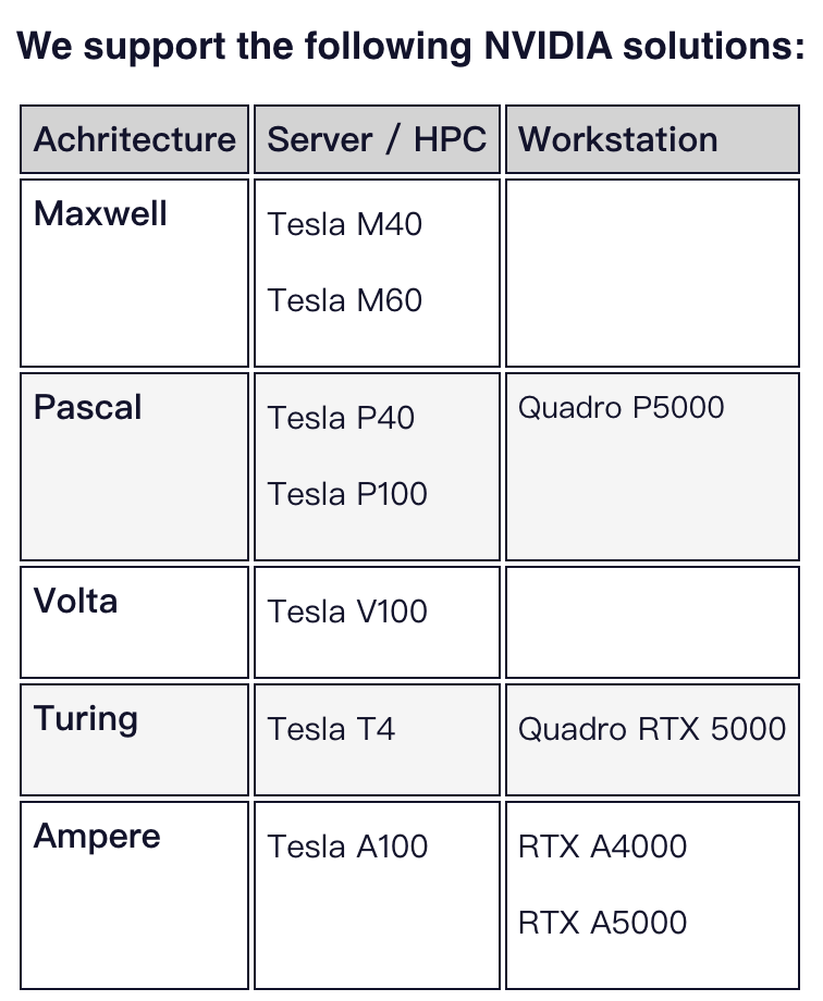
1、不支持Tesla K20、Tesla K40和Tesla K80卡。虽然我们仍然希望我们的GPGPU代码能够运行,但NVIDIA已经拒绝了CUDA 11.2工具包中对这些卡的支持。
2、我们仅支持最低CUDA版本11.2的这些卡的NVIDIA“推荐/认证”Linux驱动程序。
3、标准支持不包括消费级GPU卡,如GeForce GTX卡。
三、运行MD模拟
单次MD:
在个人笔记本(Linux)上依照上述步骤安装,或使用Windows浏览器以图形界面Web登陆HPC集群进行点击操作。
教程可参考2022薛定谔中文网络培训和知乎内容。需要注意的是:所有依赖Desmond的工作流在Windows或Mac平台上都不受支持,只能在Linux上运行。
批量MD:
1、plmd/DSMDrun: Desmond分子动力学模拟一键式运行脚本:
通过以上脚本实现当前路径下所有的mae文件(类似于PDB的结构文件,需通过Maestro转存)按照设置参数进行模拟,plmd -h中给出了示例和详细的输入命令介绍:
Usage: plmd [OPTION] <parameter>

An automatic Desmond MD pipline for protein-ligand complex MD simulation.

Example:
1) plmd -i "*.mae" -S INC -P "chain.name A" -L "res.ptype UNK" -H HPC_CPU -G HPC_GPU
2) plmd -i "*.mae" -S OUC -P "chain.name A" -L "chain.name B" -t 200 -H HPC_CPU -G HPC_gpu01
3) plmd -i "*.mae" -S "TIP4P:Cl:0.15-Na-Cl+0.02-Fe2-Cl+0.02-Mg2-Cl" -L "res.num 999" -G HPC_gpu03
4) plmd -i "*.cms" -P "chain.name A" -L "res.ptype ADP" -H HPC_CPU -G HPC_gpu04

Input parameter:
  -i	Use a file name (Multiple files are wrapped in "", and split by ' ') *.mae or *.cms ;
            or regular expression to represent your input file, default is *.mae.

System Builder parameter:
  -S    System Build Mode: <INC>
            INC: System in cell, salt buffer is 0.15M KCl, water is TIP3P. Add K to neutralize system.
            OUC: System out of cell, salt buffer is 0.15M NaCl, water is TIP3P. Add Na to neutralize system.
            Custom Instruct: Such as: "TIP4P:Cl:0.15-Na-Cl+0.02-Fe2-Cl+0.02-Mg2-Cl"
                Interactive addition of salt. Add Cl to neutralize system.
                    for positive_ion: Na, Li, K, Rb, Cs, Fe2, Fe3, Mg2, Ca2, Zn2 are predefined.
                    for nagative_ion: F, Cl, Br, I are predefined.
                    for water: SPC, TIP3P, TIP4P, TIP5P, DMSO, METHANOL are predefined.

  -b	Define a boxshape for your systems. <cubic>
            box types: dodecahedron_hexagon, cubic, orthorhombic, triclinic
  -s	Define a boxsize for your systems.  <15.0>
		for dodecahedron_hexagon and cubic, defulat is 15.0;
		for orthorhombic or triclinic box, defulat is [15.0 15.0 15.0];
		If you want use Orthorhombic or Triclinic box, your parameter should be like "15.0 15.0 15.0"
  -R    Redistribute the mass of heavy atoms to bonded hydrogen atoms to slow-down high frequency motions.
  -F	Define a force field to build your systems. <OPLS_2005>
		OPLS_2005, S-OPLS, OPLS3e, OPLS3, OPLS2 are recommended to protein-ligand systems.

Simulation control parameter:
  -m	Enter the maximum simulation time for the Brownian motion simulation, in ps. <100>
  -t    Enter the Molecular dynamics simulation time for the product simulation, in ns. <100>
  -T    Specify the temperature to be used, in kelvin. <310>
  -N    Number of Repeat simulation with different random numbers. <1>
  -P    Define a ASL to protein, such as "protein".
  -L    Define a ASL to ligand, such as "res.ptype UNK".
  -q    Turn off protein-ligand analysis.
  -u    Turn off md simulation, only system build.
  -C    Set constraint to an ASL, such as "chain.name A AND backbone"
  -f    Set constraint force, default is 10.
  -o    Specify the approximate number of frames in the trajectory.  <1000>
        This value is coupled with the recording interval for the trajectory and the simulation time: the number of frames times the trajectory recording interval is the total simulation time.
        If you adjust the number of frames, the recording interval will be modified.

Job control:
  -G	HOST of GPU queue, default is HPC_GPU.
  -H    HOST of CPU queue, default is HPC_CPU.
  -D	Your Desmond path. <$Desmond>
2、AutoMD: Desmond分子动力学模拟一键式运行脚本:
下载地址:Wang-Lin-boop/AutoMD: Easy to get started with molecular dynamics simulation. (github.com)
脚本介绍:AutoMD:从初始结构到MD轨迹,只要一行Linux命令? - 知乎 (zhihu.com)
由于Desmond学术版本提供的力场有限,plmd无法有效引入其他力场参数,因此在plmd的迭代版本AutoMD上,通过配置D.E.Shaw Research开发的Viparr和Msys代码在Desmond中引入如Amber,Charmm等力场来帮助模拟系统的构建。
在个人笔记本(Linux)上下载以下代码文件,并上传至集群个人home的software中:
wget https://github.com/DEShawResearch/viparr/releases/download/4.7.35/viparr-4.7.35-cp38-cp38-manylinux2014_x86_64.whl
wget https://github.com/DEShawResearch/msys/releases/download/1.7.337/msys-1.7.337-cp38-cp38-manylinux2014_x86_64.whl
git clone git://github.com/DEShawResearch/viparr-ffpublic.git
git clone https://github.com/Wang-Lin-boop/AutoMD
随后进入desmond工作目录,启动虚拟环境以帮助安装Viparr和Msys:
cd /fsa/home/ljx_zhangzw/software
./run schrodinger_virtualenv.py schrodinger.ve
source schrodinger.ve/bin/activate
pip install --upgrade pip
pip install msys-1.7.337-cp38-cp38-manylinux2014_x86_64.whl
pip install viparr-4.7.35-cp38-cp38-manylinux2014_x86_64.whl
echo "export viparr=${PWD}/schrodinger.ve/bin" >> ~/.bashrc
同时,将viparr-ffpublic.git解压并添加到环境变量:
echo "export VIPARR_FFPATH=${PWD}/viparr-ffpublic/ff" >> ~/.bashrc最后,将AutoMD.git解压并进行安装,同时指定可自动添加补充力场:
cd AutoMD
echo "alias AutoMD=${PWD}/AutoMD" >> ~/.bashrc
chmod +x AutoMD
source ~/.bashrc
cp -r ff/* ${VIPARR_FFPATH}/
#AutoMD -h
在输入命令介绍中,给出了四个示例:胞质蛋白-配体复合物、血浆蛋白-蛋白复合物、DNA/RNA-蛋白质复合物、以及需要Meastro预准备的膜蛋白。在这些示例中:
通过-i命令输入了当前路径所有的复合物结构.mae文件(也可以是Maestro构建好的模拟系统.cms文件);
通过-S指定了模拟系统的溶液环境,包括INC(0.15M KCl、SPC水、K+中和)、OUC(0.15M NaCl、SPC水、Na+中和),以及自定义溶液环境如"SPC:Cl:0.15-K-Cl+0.02-Mg2-Cl";
通过-b和-s定义了模拟系统的Box形状和大小;
通过-F定义力场参数,由于学术版Desmond的要求不被允许使用S-OPLS力场,仅可使用OPLS_2005或其他力场;OPLS适用于蛋白-配体体系,Amber适用于蛋白-核酸,Charmm适用于膜蛋白体系,DES-Amber适用于PPI复合体体系,但是这些搭配并不是绝对的,我们当然也可以尝试在膜蛋白体系上使用Amber力场,在核酸体系上使用Charmm力场,具体的情况需要用户在自己的体系上进行尝试;
| -F Charmm ff | aa.charmm.c36m, misc.charmm.all36, carb.charmm.c36, ethers.charmm.c35, ions.charmm36, lipid.charmm.c36 and na.charmm.c36 |
| -F Amber ff | aa.amber.19SBmisc, aa.amber.ffncaa, lipid.amber.lipid17, ions.amber1lm_iod.all, ions.amber2ff99.tip3p, na.amber.bsc1 and na.amber.tan2018 |
| -F DES-Amber | aa.DES-Amber_pe3.2, dna.DES-Amber_pe3.2, rna.DES-Amber_pe3.2 and other force fields in -F Amber |
Usage: AutoMD [OPTION] <parameter>

Example:
1) MD for cytoplasmic protein-ligand complex:
AutoMD -i "*.mae" -S INC -P "chain.name A" -L "res.ptype UNK" -F "S-OPLS"
2) MD for plasma protein-protein complex:
AutoMD -i "*.mae" -S OUC -F "DES-Amber"
3) MD for DNA/RNA-protein complex:
AutoMD -i "*.mae" -S "SPC:Cl:0.15-K-Cl+0.02-Mg2-Cl" -F Amber
4) MD for membrane protein, need to prior place membrane in Meastro.
AutoMD -i "*.mae" -S OUC -l "POPC" -r "Membrane" -F "Charmm"

Input parameter:
  -i    Use a file name (Multiple files are wrapped in "", and split by ' ') *.mae or *.cms ;
            or regular expression to represent your input file, default is *.mae.

System Builder parameter:
  -S    System Build Mode: <INC>
        INC: System in cell, salt buffer is 0.15M KCl, water is SPC. Add K to neutralize system.
        OUC: System out of cell, salt buffer is 0.15M NaCl, water is SPC. Add Na to neutralize system.
        Custom Instruct: Such as: "TIP4P:Cl:0.15-Na-Cl+0.02-Fe2-Cl+0.02-Mg2-Cl"
            Interactive addition of salt. Add Cl to neutralize system.
                for positive_ion: Na, Li, K, Rb, Cs, Fe2, Fe3, Mg2, Ca2, Zn2 are predefined.
                for nagative_ion: F, Cl, Br, I are predefined.
                for water: SPC, TIP3P, TIP4P, TIP5P, DMSO, METHANOL are predefined.
  -l    Lipid type for membrane box. Use this option will build membrane box. <None>
            Lipid types: POPC, POPE, DPPC, DMPC.
  -b    Define a boxshape for your systems. <cubic>
            box types: dodecahedron_hexagon, cubic, orthorhombic, triclinic
  -s    Define a boxsize for your systems.  <15.0>
            for dodecahedron_hexagon and cubic, defulat is 15.0;
            for orthorhombic or triclinic box, defulat is [15.0 15.0 15.0];
            If you want use Orthorhombic or Triclinic box, your parameter should be like "15.0 15.0 15.0"
  -R    Redistribute the mass of heavy atoms to bonded hydrogen atoms to slow-down high frequency motions.
  -F    Define a force field to build your systems. <OPLS_2005>
            OPLS_2005, S-OPLS are recommended to receptor-ligand systems.
            Amber, Charmm, DES-Amber are recommended to other systems. Use -O to show more details.
            Use the "Custom" to load parameters from input .cms file.

Simulation control parameter:
  -m    Enter the maximum simulation time for the Brownian motion simulation, in ps. <100>
  -r    The relaxation protocol before MD, "Membrane" or "Solute". <Solute>
  -e    The ensemble class in MD stage, "NPT", "NVT", "NPgT". <NPT>
  -t    Enter the Molecular dynamics simulation time for the product simulation, in ns. <100>
  -T    Specify the temperature to be used, in kelvin. <310>
  -N    Number of Repeat simulation with different random numbers. <1>
  -P    Define a ASL to receptor, such as "protein".
  -L    Define a ASL to ligand and run interaction analysis, such as "res.ptype UNK".
  -u    Turn off md simulation, only system build.
  -C    Set constraint to an ASL, such as "chain.name A AND backbone"
  -f    Set constraint force, default is 10.
  -o    Specify the approximate number of frames in the trajectory.  <1000>
        This value is coupled with the recording interval for the trajectory and the simulation time:
        the number of frames times the trajectory recording interval is the total simulation time.
        If you adjust the number of frames, the recording interval will be modified.

Job control:
  -G    HOST of GPU queue, default is GPU.
  -H    HOST of CPU queue, default is CPU.
  -D    Your Desmond path. </fsa/home/ljx_zhangzw/>
  -V    Your viparr path. </fsa/home/ljx_zhangzw/schrodinger.ve/bin>
-v Your viparr force fields path. </fsa/home/ljx_zhangzw/viparr-ffpublic/ff>示例任务提交脚本及命令,需修改相应计算节点和软件路径信息:
#BSUB -L /bin/bash
#BSUB -q 83a100ib
#BSUB -m m001
module load cuda/12.0.0
export Desmond=/fsa/home/ljx_zhangzw/
export viparr=/fsa/home/ljx_zhangzw/schrodinger.ve/bin
export VIPARR_FFPATH=/fsa/home/ljx_zhangzw/viparr-ffpublic/ff
alias AutoMD=/fsa/home/ljx_zhangzw/AutoMD/AutoMD
echo $PATH
echo $LD_LIBRARY_PATH
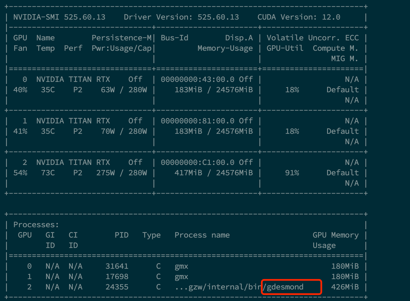
nvidia-smi
env|grep CUDA
AutoMD -i "*.mae" -S OUC -P "chain.name A" -L "res.ptype UNK" -F "OPLS_2005" -T 298 -s 10 -H m001 -G m001在模拟参数控制命令中,通过-P和-L分别定义了mae文件中的受体和配体,-m默认
-T定义体系温度为298 K,默认进行100 ns和1次重复模拟次数,通过-H和-G指定了host文件中的相应计算队列。
四、性能表现:
笔者通过上述的示例任务提交脚本及命令调用Desmond和AutoMD进行了包含12个阶段的工作流:
Summary of user stages:
  stage 1 - task
  stage 2 - build_geometry
  stage 3 - assign_forcefield
  stage 4 - simulate, Brownian Dynamics NVT, T = 10 K, small timesteps, and restraints on solute_heavy_atom, 100 ps
  stage 5 - simulate, Brownian Dynamics NVT, T = 10 K, small timesteps, and restraints on user defined sets, 100 ps
  stage 6 - simulate, Langevin small steps NVT, T = 10 K, and restraints on solute heavy atoms, 12 ps
  stage 7 - simulate, Langevin NPT, T = 10 K, and restraints on solute heavy atoms, 12 ps
  stage 8 - simulate, Langevin NPT, T = 10 K, and restraints on solute heavy atoms, 12 ps
  stage 9 - simulate, Langevin NPT and restraints on solute heavy atoms, 12ps
  stage 10 - simulate, Langevin NPT and no restraints, 24ps
  stage 11 - simulate, Final MD and analysis, 100000.0 ps
  stage 12 - pl_analysis
(12 stages in total)
分别在83a100ib和72rtxib进行了相应尝试:
System Atoms:21173
System Residues:6363
System MOls:6202
Protein Atoms:2584
Protein Residues:162
Ligand Atoms:73
Ligand Residues:1


MIN time: 100 ps
MD time: 100000.0 ps
temperature: 298 K
Repeat: 1
Rondom numbers list: 2007

#Desmond
Multisim summary :
Total duration: 3h 38' 7"
Total GPU time: 3h 24' 42" (used by 8 subjob(s))

#HPC-83a100ib
Resource usage summary:

    CPU time :                                   12745.00 sec.
    Max Memory :                                 965 MB
    Average Memory :                             893.78 MB
    Total Requested Memory :                     -
    Delta Memory :                               -
    Max Swap :                                   -
    Max Processes :                              15
    Max Threads :                                45
    Run time :                                   13262 sec.
    Turnaround time :                            13260 sec.
System Atoms:63284
System Residues:20178
System MOls:19955
Protein Atoms:2585
Protein Residues:224
Ligand Atoms:72
Ligand Residues:1
MIN time: 100 ps
MD time: 100000.0 ps
temperature: 298 K
Repeat: 1
Rondom numbers list: 2007
#Desmond
Multisim summary :
Total duration: 7h 51' 5"
Total GPU time: 7h 27' 48" (used by 8 subjob(s))
#HPC-72rtxib
Resource usage summary:
CPU time : 31316.00 sec.
Max Memory : 1634 MB
Average Memory : 400.16 MB
Total Requested Memory : -
Delta Memory : -
Max Swap : -
Max Processes : 15
Max Threads : 40
Run time : 85601 sec.
Turnaround time : 85602 sec.笔者在测试时恰逢72rtxib g007中有同学在运行gmx,desmond的GPU利用率得到了进一步的凸显,但目前存在一点问题,即desmond在计算完毕后无法及时退出对GPU的占用,
***我将在错误解决后更新,或者如果你知道如何排除这个出错误,请在QQ群探讨***
五、模拟分析:
模拟完成后,将在工作路径创建一个名为结构文件名_随机种子号-md的文件夹,其中包含了:
| 多个阶段的工作流文件 | AutoMD.msj |
| 多个阶段 launching日志文件 | md_multisim.log |
| 多个阶段 launching阶段文件 | md_1-out.tgz ... md_12-out.tgz |
| 模拟系统结构文件 | -in.cms and -out.cms |
| 模拟执行参数文件 | md.cpt.cfg and md-out.cfg |
| 模拟轨迹文件夹 | md_trj |
| 模拟执行日志文件 | md.log |
| 检查点文件 | md.cpt |
| 能量文件 | md.ene |
| 包含RMSF、RMSF、SSE等常规分析的结果文件 | md.eaf |
此外,还包含了部分的分析脚本文件,更多用于MD轨迹分析的脚本文件还可以通过访问官方脚本库获得Scripts | Schrödinger (schrodinger.com);
| 文件夹内分析脚本 | |
| Resume previous MD | bash resume.sh |
| Extend MD | bash extend.sh # The total time will be extend to 2-fold of initial time |
| Cluster trajectory | bash cluster.sh "<rmsd selection>" "<fit selection>" "<number>" |
| Analysis Occupancy | bash occupancy.sh "<selection to analysis>" "<fit selection>" |
| Analysis ppi contact | bash ppi.sh "<Component A>" "<Component B>" |
| 官网部分MD脚本 | |
| Calculate the radius of gyration | calc_radgyr.py |
| Thermal MMGBSA |
thermal_mmgbsa.py |
| Calculate Trajectory B-factors |
trajectory_bfactors.py |
| Analyze a Desmond Simulation |
analyze_simulation.py |
| Merge Trajectories |
trj_merge.py |
上述分析脚本的使用需预先设置环境变量,随后在terminal键入$SCHRODINGER/run *.py -h查看相应脚本的帮助文件即可,如在个人计算机 (LINUX)中进行轨迹80-100ns的mmgbsa计算分析:
vim ~/.bashrc
#添加schrodinger所在目录的环境变量:
export SCHRODINGER=/opt/schrodinger2018-1
source ~/.bashrc
#执行80-100 ns的mmgbsa计算,间隔4帧
$SCHRODINGER/run thermal_mmgbsa.py *-2007-md-out.cms -j casein80_100 -start_frame 800  -end_frame 1000  -HOST localhost:8 -NJOBS 4 -step_size 4
结合thermal_mmgbsa.py的计算结果,breakdown_MMGBSA_by_residue.py脚本进一步实现了mmgbsa结合能的残基分解:
$SCHRODINGER/run breakdown_MMGBSA_by_residue.py *-prime-out.maegz *-breakdown.csv -average结合thermal_mmgbsa.py产生所有帧的结构文件:MD_0_100ns-complexes.maegz,使用calc_radgyr.py脚本计算复合物的回旋半径:
$SCHRODINGER/run calc_radgyr.py -h
#usage: calc_radgyr.py [-v] [-h] [-asl ASL] infile

Calculates the radius of gyration of structures in the input file.

Calculate the radius of gyration of each structure in the input file,
which can be Maestro, SD, PDB, or Mol2 format.

Copyright Schrodinger, LLC. All rights reserved.

positional arguments:
  infile        Input file.

optional arguments:
  -v, -version  Show the program's version and exit.
  -h, -help     Show this help message and exit.
  -asl ASL      ASL expression for atoms to be included in the calculation. By
                default, the radius of gyration includes all atoms.
#示例
$SCHRODINGER/run thermal_mmgbsa.py *-2007-md-out.cms -j * -start_frame 0  -end_frame 1001  -HOST localhost:8 -NJOBS 4 -step_size 1
$SCHRODINGER/run calc_radgyr.py *-2007-md-out.cms
结合binding_sasa.py脚本实现复合物的SASA分析:
$SCHRODINGER/run binding_sasa.py -h
#usage: binding_sasa.py [-v] [-h] [-r RESIDUES] [-d <angstrom distance> | -f] [-s] [-n]
[-o OUTPUT_FILE] [-l ASL] [-j JOBNAME]
[--trajectory <path to trj>] [--ligand_asl <ligand asl>]
[--framestep <frames in each step>]
[--water_asl <asl for waters to keep>]
input_file
Calculates SASA of ligand and receptor before and after receptor-ligand binding.
Computes the change in solvent accessible surface area (SASA) upon binding for
a ligand and receptor. The total SASA for the unbound system and the
difference upon binding is computed and decomposed into functional subsets,
such as per-residue terms, charged, polar, and hydrophobic
The script will operate on PV files, Desmond CMS files or a receptor-ligand
complex Maestro file.
Copyright Schrodinger, LLC. All rights reserved.
positional arguments:
input_file Input PV file, Desmond CMS file, or a receptor-ligand complex
Maestro file.
optional arguments:
-v, -version Show the program's version and exit.
-h, -help Show this help message and exit.
-r RESIDUES, --residue RESIDUES
Add specific residue to SASA report. Can be done multiple times
to add multiple residues. (format: ChainID,ResNum)
-d <angstrom distance>, --distance <angstrom distance>
Distance cutoff in angstroms. Receptor atoms further than
cutoff distance from ligand will not be included in protein-
ligand complex SASA calculation. Default is 5 angstroms.
-f, --full Calculates SASA for entire ligand and protein.
-s, --structure For each ligand and receptor, append additional output
reporting the surface area of backbone atoms, side chain atoms,
and atoms of each residue type.
-n, --secondary For each ligand and receptor, append additional output
reporting surface area for helix , strand and loop receptor
atoms.
-o OUTPUT_FILE, --output OUTPUT_FILE
Where to write the output file. If not specified, for PV input,
output file will be called <jobname>_out_pv.mae; for complex
files, it will be named <jobname>-out.mae. For --trajectory
jobs, only CSV output file is written
-l ASL, --selection ASL
ASL pattern to define specific residues to calculate SASA for.
-j JOBNAME, --jobname JOBNAME
Sets the jobname - base name for output files. If not
specified, it will be derived from the input file name.
--trajectory <path to trj>
Compute binding SASA over a trajectory. Use of this option
means the input file should be a Desmond .cms file. The path to
the Desmond trj directory must be supplied as the argument to
this flag. Output will be to a .csv file only. The ligand
structure will be determined automatically unless the
--ligand_asl flag is used.
--ligand_asl <ligand asl>
The ASL used to determine the ligand structure. By default,
this is determined automatically. Only valid for --trajectory
jobs.
--framestep <frames in each step>
--trajectory jobs calculate SASA every X frames. By default,
X=10. Use this flag to change the value of X.
--water_asl <asl for waters to keep>
By default, --trajectory jobs remove all waters before
calculating SASA. Use this to specify waters to keep
(--water_asl=all keeps all waters, --water_asl="within 5
backbone" keeps all waters with 5 Angstroms of the protein
backbone).
#示例
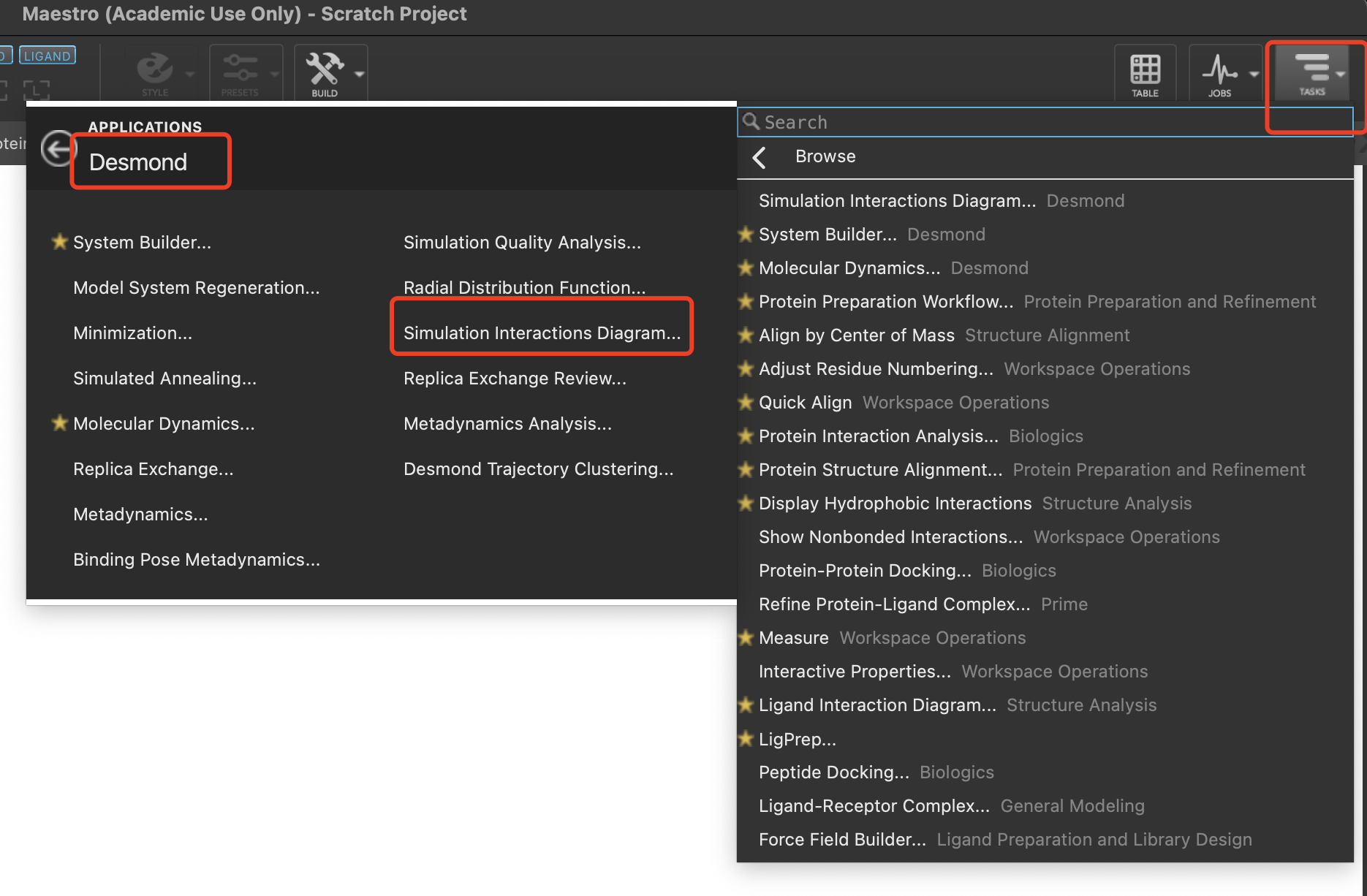
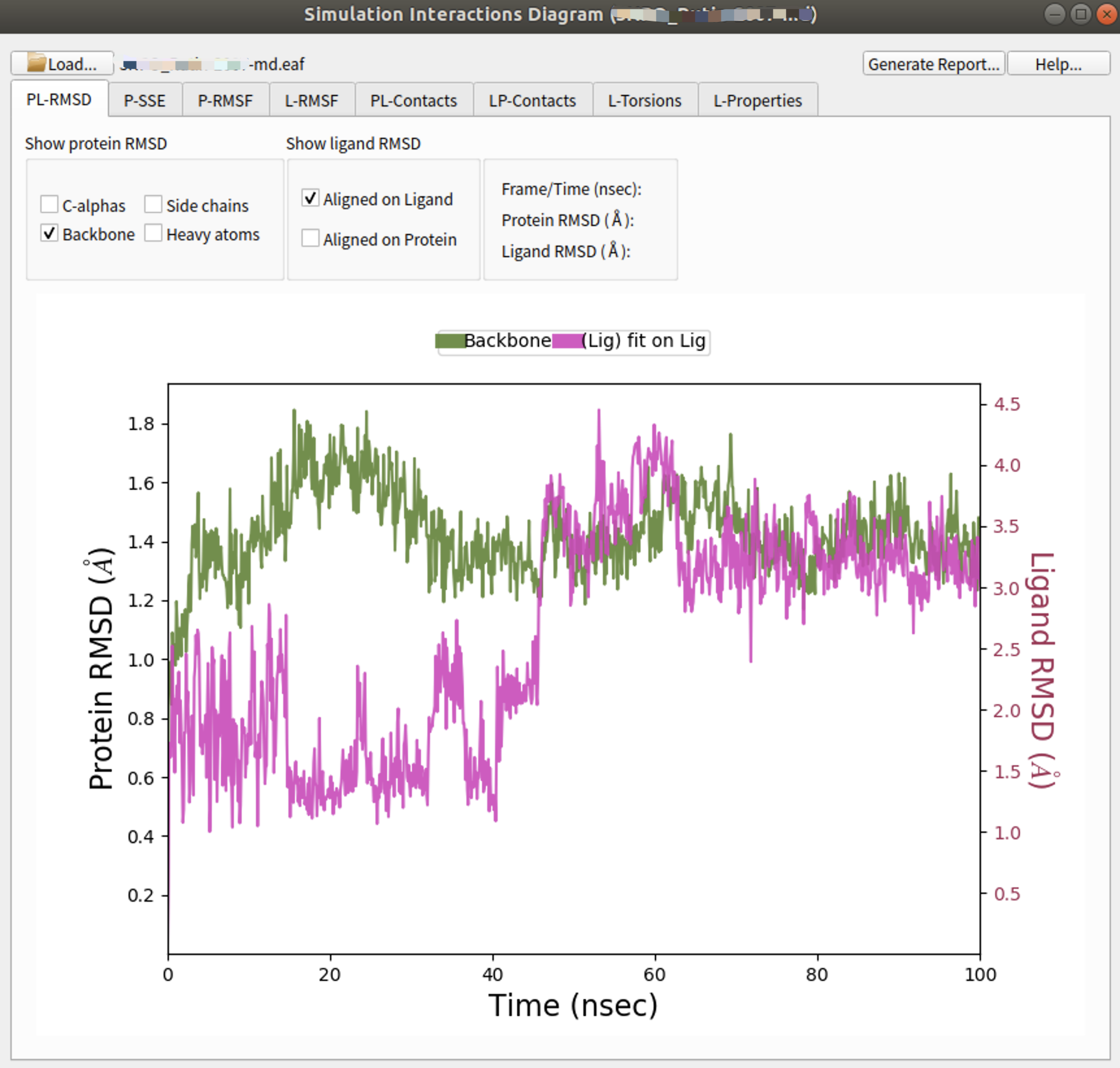
$SCHRODINGER/run binding_sasa.py *-2007-md-out.cms -f -j sasa_complex --trajectory *-2007-md_trj --framestep 1还可以通过下载结构文件名_随机种子号-md的文件夹至个人笔记本,在TASKS中的Desmond找到Simulation Interaction Digram分析面板,并导入md.eaf文件进行常规分析。
借助AutoMD中的AutoTRJ脚本,可以使用常见的官方脚本来直接处理AutoMD的模拟结果:
(base) parallels@parallels:$ AutoTRJ -h
The trajectory analysis script for AutoMD. Refer to: https://github.com/Wang-Lin-boop/AutoMD
Usage: AutoTRJ [OPTION] <parameter>

Required Options:
  -i <string>	The path to trajectory or regular expression for trajectories(will be merged). such as "*-md".
  -J <string>   Specify a basic jobname for this task, the basename of -i is recommended.
  -M <string>   The running mode for this analysis task. the <..> means some options.
                APCluster_<n>: affinity propagation clustering, the <n> is the number of most populated clusters.
                CHCluster_<n>_<cutoff>: centroid hierarchical clustering, the <cutoff> is the RMSD thethreshold.
                LigandAPCluster_<n>: APCluster for ligand, require "-L" option.
                LigandCHCluster_<n>_<cutoff>: CHCluster for ligand, require "-L" option.
                Occupancy: calculates the occupancy of component 2 in trajectory, require "-L" option.
                PPIContact: identifies interactions occurring between the components, require "-L" option.
                FEL: analyze the free energy landscape (FEL) for CA atoms, and cluster the trajectories by FEL.
                CCM: plot the cross-correlation matrix of the trajectory.
                SiteMap_<n>: running SiteMap on all frames of the trajectory, the <n> is the number of sites.
                PocketMonitor: monitor the ligand binding pocket on the trajectory, require "-L" option.
                MMGBSA: running MM-GBSA on the trajectory, require "-L" option.
                BFactor: calculate atom B-factors from trajectory (receptor and ligand).
                RMSF: calculate RMSF from trajectory (receptor).
                ConvertXTC: convert the trajectory to XTC format.
            You can parallel the analysis task by "+", such as, "APCluster_5+PPIContact+MMGBSA".

Analysis Range Options:
  -R <ASL>      The ASL of component 1 to be centered. <protein>
  -L <ASL>      The ASL of component 2 to be analyzed. <ligand>

Trajectories Processing Options:
  -T <string>   Slice trajectories when analyzed, if more than one trajectories given by -i, this slice will applied to all of them. The default is None. Such as "100:1000:1". <START:END:STEP>
  -t <string>   Slice trajectories when calculating MM/GBSA, such as "100:1000:1". <START:END:STEP>
  -c            During the clustering process, the frames of a trajectory are preserved for each cluster, while representative members are stored in the CMS files.
  -A <file>     Align the trajectory to a reference structure, given in ".mae" format.
  -a            Align the trajectory to the frist frame.
  -C <ASL>      Set a ASL to clean the subsystem from trajectory, such as -C "not solvent".
  -P            Parch waters far away from the component 2.
  -w <int>      Number of retained water molecules for parch (-P) stage. <200>
  -m            Treat the explicit membrane to implicit membrane during MM-GBSA calculation.

Job Control Options:
  -H <string>   HOST of CPU queue, default is CPU.与Desmond配置schrondinger.host相同
  -N <int>      CPU number for per analysis task. <30>
  -G <path>     Path to the bin of Gromacs. <此处填写Gromacs的路径>
  -D <path>	    Path to the installation directory of Desmond. <此处填写Desmond或Schrodinger的路径>
#示例
AutoTRJ -i *-md_trj -J test_xpm -M FEL -G /usr/local/gromacs/bin/
#此处输入了md的轨迹文件,并指定分析人物名称为test_xpm,分析任务为FEL,额外指定了gmx的环境变量(由于在我自己的虚拟机上)
六、致谢:
需要强调的是,AutoMD是一个建立在Desmond软件包基础上的脚本,模拟的质量由Desmond本身决定,脚本没有对模拟程序本身做任何的改动,且所有的学术贡献归功于D. E. Shaw Research (无商业利益相关)。
AutoMD作为一个使用脚本,仅仅是为了解决了一些实际MD应用中的问题,方便初学者通过这个脚本快速上手MD,但请勿认为AutoMD是一种MD模拟的程序,其内核仍然是Desmond程序。
本文所有内容均来自上海科技大学Wang-Lin,笔者整理使用经验而已。
请大家多多引用作者关于 AutoMD脚本的文章:A new variant of the colistin resistance gene MCR-1 with co-resistance to β-lactam antibiotics reveals a potential novel antimicrobial peptide. Liang L, Zhong LL, Wang L, Zhou D, Li Y, et al. (2023) A new variant of the colistin resistance gene MCR-1 with co-resistance to β-lactam antibiotics reveals a potential novel antimicrobial peptide. PLOS Biology 21(12): e3002433. https://doi.org/10.1371/journal.pbio.3002433
集群运行Numpy程序的测试实践与注意事项
你正确安装Numpy了吗?
本测试主要使用的是某Numpy为底层的计算包,任务的核心在于求解矩阵对角化,使用的是LAPACK。计算的大头在于500次尺寸约为60000×60000的稀疏矩阵对角化计算。
从不同渠道安装的Numpy,其所使用的LAPACK优化可能并不一样,在不同的硬件上性能表现也大不相同。常见的优化有MKL、OpenBLAS和ATLAS,其中通常说来Intel的CPU上跑MKL会更快一些。
一般来说,不考虑指定渠道,默认情况下
conda install numpy
从Anaconda下载安装会根据你的CPU自动选择,若是Intel则用MKL,若是AMD则用OpenBLAS。当然,你可以切换到conda-forge之类的去指定版本。
如果使用pip安装,
pip install numpy
则一律是OpenBLAS。
MKL的插曲
测试最初采用MKL版Numpy计算,通过环境变量MKL_NUM_THREADS这个环境变量设定不同的核数控制多线程计算(这是使用Numpy等存在隐性并行的库都需要注意的,参考常见问题-作业运行时实际占用CPU核数过多),在同一队列提交多个独占节点的计算任务。
MKL大多数情况下都比OpenBLAS快,即便是在AMD平台上也有传说中的MKL_DEBUG_CPU_TYPE=5可以强开对MKL的支持。
但是,本次测试却出现了非常有趣的现象:
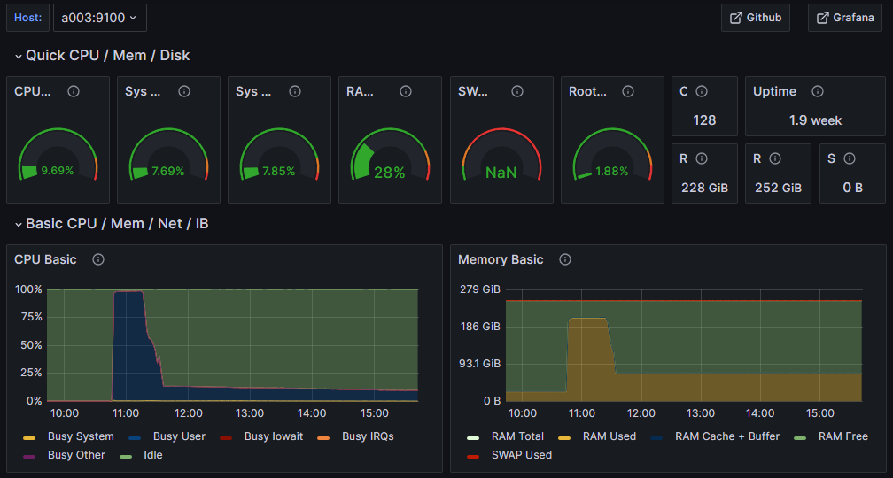
通过eScience中心的监控系统查看节点计算情况,发现大多数进程都陆陆续续计算完毕,平均在40分钟左右;而少数任务,例如最初申请了16核,突然在40分钟前后发现线程数急剧减少至单核或少量核,出现“一核有难,多核围观”的经典场面,内存也被释放掉了。但是主要的计算阶段仍然没有输出计算结果说明并不是核心计算完成陷入单线程无法结束的问题。
最终计算完成的时间统计也剧烈起伏。经过网上的一通搜索,并未发现很多案例。作为猜测,将其它的LAPACK优化库限制核数加入,都没有改善。更换AMD队列,仍然是同样的问题。也就是说,这个情况的出现与是Intel还是AMD的CPU没有关系。
然而最终,尝试性更换至OpenBLAS版本Numpy,发现问题神奇地解决了。
多核情况测试
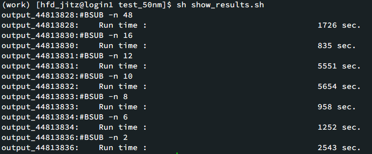
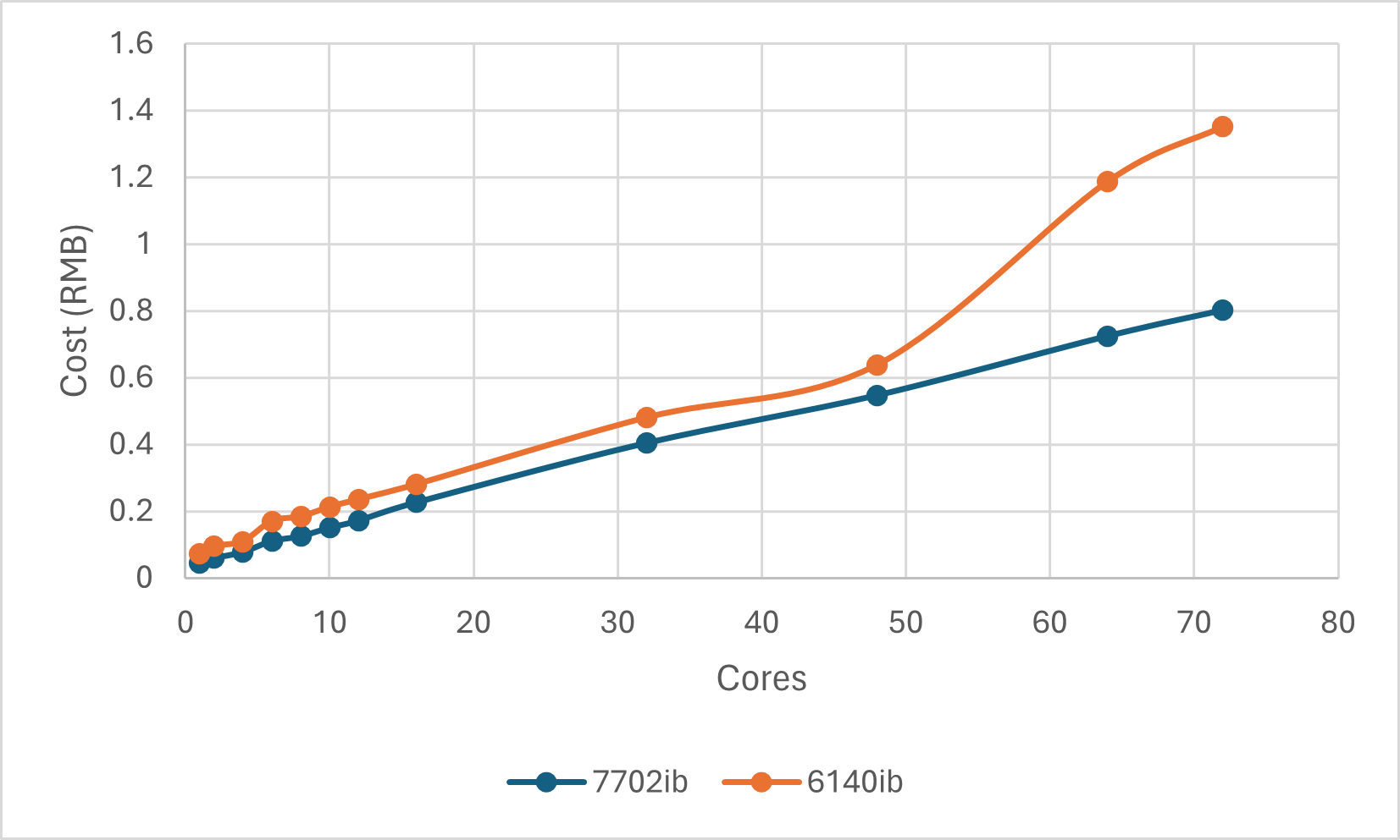
由于MKL版本的神秘BUG,后来的测试通过OpenBLAS版本进行。多核计算单个任务的总耗时结果如下:
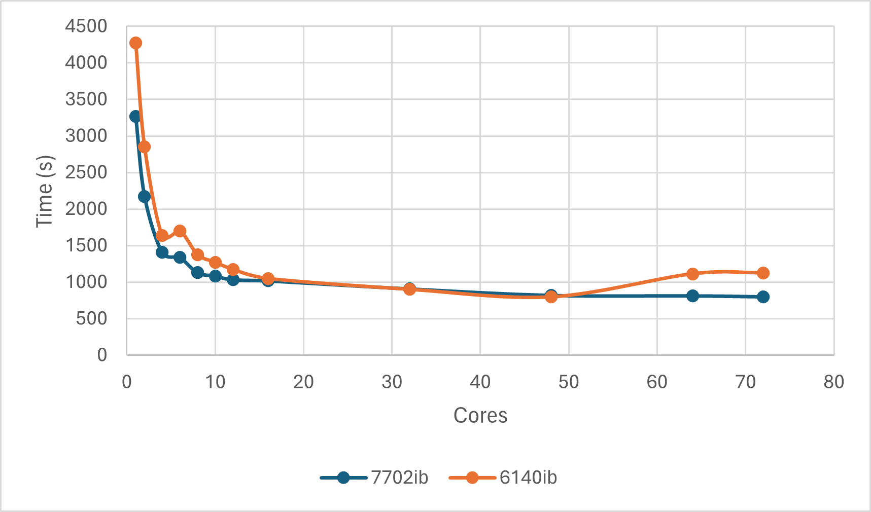
可以发现,OpenBLAS版Numpy的计算在7702ib队列和6140ib在48核以下的趋势类似,但高于48核不太一样。7702ib队列上核数越多相对而言加速的趋势一致;而6140ib队列上,核数越多反而可能会有加速效果的下降。但由于7702ib的核数更多,因此并不能排除核数大于72时也会有类似的情况。
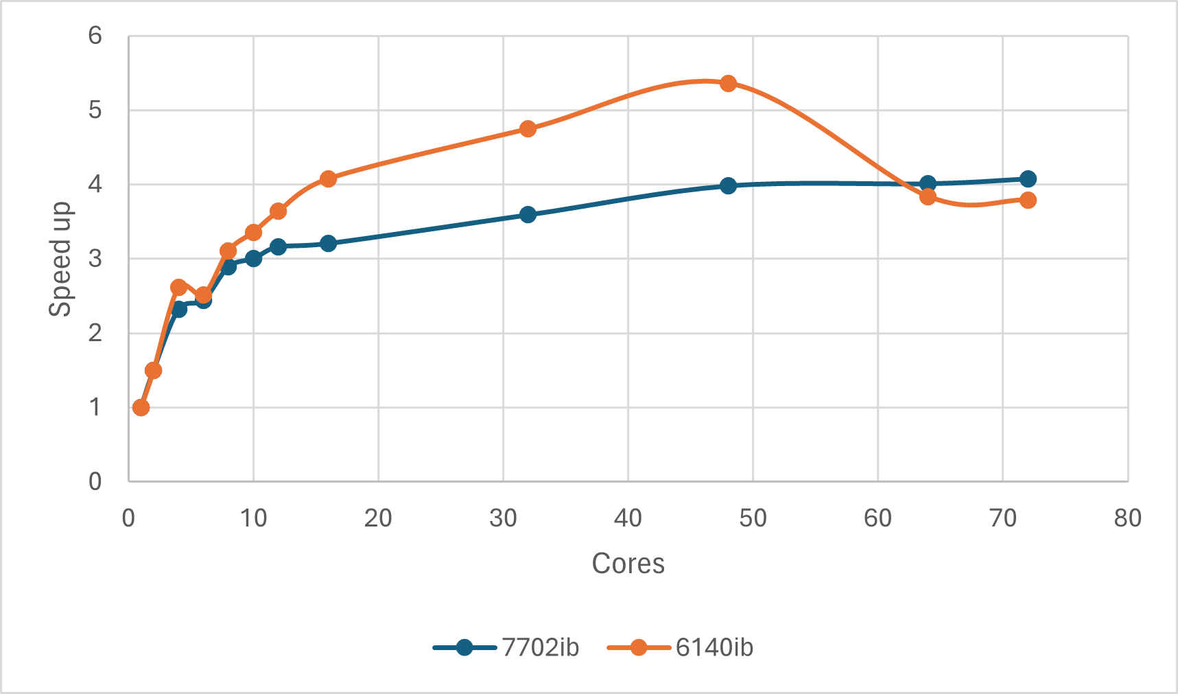
从加速比(相对串行计算的时间比值)来看,对于本测试任务,OpenBLAS Numpy的加速比极限约为4~5倍。
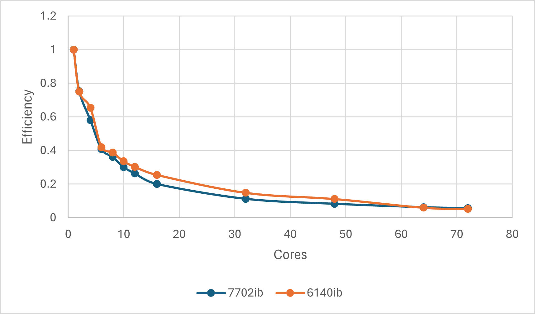
并行效率(相对串行计算的时间比值再除以核数)则随核数增多衰减极快,16核往上效率极低,全靠数量取胜。
投放任务的策略
对单个任务来说,我们只关心这一次计算的时间,因此时间肯定是越短越好。但是往往时间和核数(准确来说是申请CPU乘以时间)影响计算费用,因此计算核时的指标额外决定了是否划算。根据收费办法我们可以画出实际的花费。显然有些队列上有时候申请过多的核并不一定是划算的,这也是做基准测试的意义所在。
更多时候,我们可能面对的是多个计算量相当的任务,只是计算参数不同。这种情况下,我们可以根据下列公式计算:
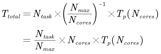
其中,N_task 指的是总任务数,N_max指的是考虑申请的总核数,N_cores指的是单个任务申请的核数,T_p是单个任务并行计算的耗时,与单个任务申请的核数有关系。N_cores与T_p相乘即为单个任务的计算核时。
可以看到,总的核时(T_total乘以N_max)也和上文的单个任务类似。
单从性价比而言,不同的核数下,我们对单个任务每加速一倍花了多少钱,也可以算出:
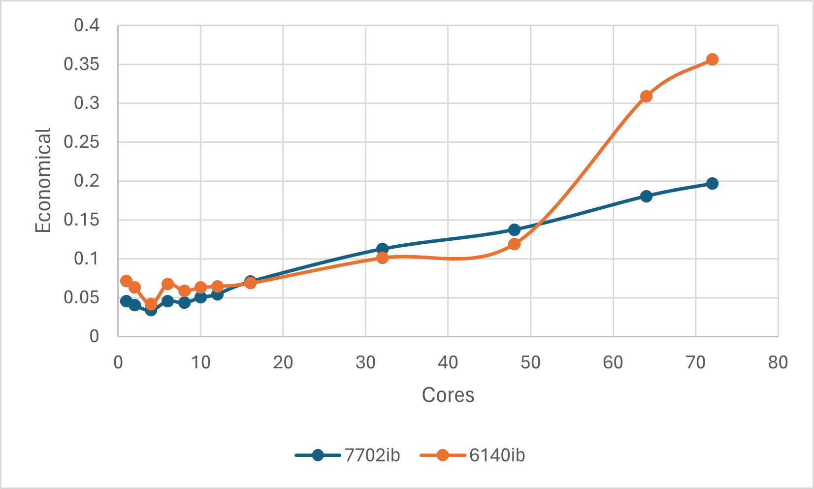
对于Numpy(OpenBLAS)计算本任务而言,性价比最高的莫过于4核。因此综合考虑时间、性价比,4核是个不错的选择。
总结
本次尝试使用集群对Numpy计算进行加速。在尝试过程中,发现需要注意几个问题:
- Numpy(并行版本)是隐性并行,所以也需要有特定的环境变量来控制与申请核数匹配,不然会被作业监控杀掉。
- 基于MKL版Numpy或者调用Numpy的计算包计算时,出现了突然任务变慢的情况,而且会长时间不结束。这与LAPACK优化库(MKL或OpenBLAS或者其他)同当前计算包的兼容性可能有关系,如果发现类似情况,可以尝试排除此类软件依赖的数值计算库是否存在这样的不同优化(甚至编译方式)的区别。
- Numpy的并行计算存在一个加速效果的上限,对本次测试的任务来说约为4~5倍。从时间、性价比的角度来说,并非核数越多越划算,例如本任务中,较为经济而且时间可接受的一个合理范围为4~16核,其中4核最具性价比;对单个任务,其花费可能尚可,但是日积月累也许是笔不小的数目。